As retrieval-augmented generation (RAG), multimodal search engines, and semantic recommendation systems scale into hundreds of millions of embeddings, backend engineers face a fundamental computational bottleneck: exact nearest neighbor search in high-dimensional vector spaces is impossibly slow.
A naive linear scan (Exact $k$-NN / Flat Search) across $100\text{ million}$ vectors with $1536$ dimensions (the standard output of modern embedding models) requires evaluating billions of floating-point distance calculations for every single user query. In production, this results in multi-second latencies and massive GPU/RAM expenditures that quickly overwhelm cloud budgets.
To deliver sub-millisecond latencies at scale, modern vector databases (such as Qdrant, Milvus, pgvector, and Faiss) rely on Approximate Nearest Neighbor (ANN) indexing. Rather than computing exact distances to every point, ANN algorithms construct specialized geometric indexes that sacrifice less than $1\%$ of retrieval recall to achieve a $100\times$ to $1000\times$ speedup.
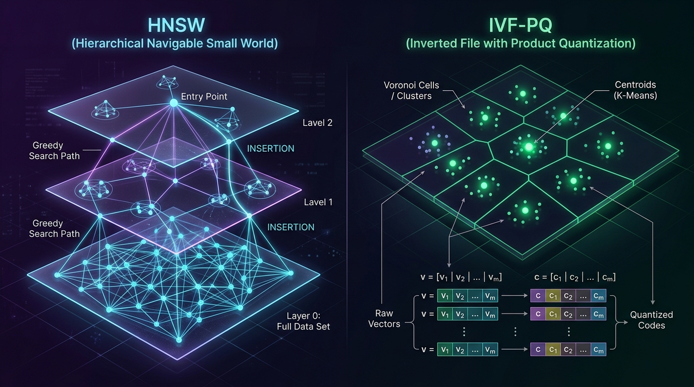
In this comprehensive guide, we dissect the internal mechanics of the two dominant vector indexing paradigms: HNSW (Hierarchical Navigable Small World) and IVF-PQ (Inverted File with Product Quantization). We will explore how they navigate high-dimensional manifolds, analyze their memory footprints and recall-vs-QPS trade-offs, and demonstrate how to optimize their parameters in production systems.
The Geometric Dilemma: Why Exact Search Fails at Scale
In low-dimensional spaces (e.g., 2D or 3D cartographic data), spatial indexes like $k$-d trees or $R$-trees partition space hierarchically to prune search regions in $O(\log N)$ time. However, when dimensionality ($D$) scales to $768$, $1536$, or $3072$, spatial partitioning collapses due to the Curse of Dimensionality.
The Geometry of High-Dimensional Space
In high dimensions, volume concentrates almost entirely in a thin outer shell near the boundary of the hypersphere, and random vectors become nearly orthogonal to one another. As a result, the distance between any arbitrary pair of points converges to almost the exact same value:
$$\lim_{D \to \infty} \frac{\text{dist}_{\max} - \text{dist}_{\min}}{\text{dist}_{\min}} \to 0$$
Spatial bounding boxes in tree algorithms end up intersecting virtually all partitions, forcing $k$-d trees to inspect almost every branch and degenerating back into an exhaustive $O(N \cdot D)$ linear scan.
Raw Memory Consumption: Flat Storage Math
Let us calculate the uncompressed RAM requirements for storing raw IEEE 754 32-bit floating-point vectors ($4\text{ bytes per dimension}$):
| Dataset Size ($N$) | Dimensions ($D = 768$) | Dimensions ($D = 1536$) | Dimensions ($D = 3072$) |
|---|---|---|---|
| 100,000 vectors | 307.2 MB | 614.4 MB | 1.23 GB |
| 1,000,000 vectors | 3.07 GB | 6.14 GB | 12.28 GB |
| 10,000,000 vectors | 30.7 GB | 61.4 GB | 122.8 GB |
| 100,000,000 vectors | 307.2 GB | 614.4 GB | 1.23 TB |
When you account for index graph pointers, metadata payload storage, and inverted lists, housing 50M+ vectors entirely in uncompressed RAM becomes economically unviable without compression and approximate indexing techniques.
HNSW (Hierarchical Navigable Small World): Graph-Based Speed and Precision
Hierarchical Navigable Small World (HNSW) is currently the golden standard for production vector search when maximum recall ($>98\%$) and ultra-low latency ($< 5\text{ms}$) are the primary system requirements.
The Core Concept: Navigable Small World & Skip-Lists
HNSW generalizes two classical computer science concepts into multi-dimensional metric spaces:
- Navigable Small World (NSW) Graphs: Networks where the average shortest path between any two vertices scales logarithmically ($\approx \log N$) with the number of nodes, characterized by high local clustering and sparse long-range highway edges (the "six degrees of separation" principle).
- Skip-Lists: Multi-level probabilistic data structures where higher layers contain sparse elements for rapid long-range navigation, while bottom layers contain all elements for granular traversal.
HNSW Multi-Layer Search Traversal:

Layer 2 (Top Sparse Layer)
[Entry Point: v8] ---------(Long-Range Jump)---------> [v42]
       |                                                 |
       v (Descend to Layer 1)                            v
Layer 1 (Medium Density Layer)
     [v8] -----> [v19] -----> [v31] -----> [v42] -----> [v78]
                                              |
                                              v (Descend to Layer 0)
Layer 0 (Full Granular Graph - All Vectors)
     [v1] <-> [v12] <-> [v31] <-> [v37] <-> [v42] <-> [v63] <-> [v78] <-> [Target]
The HNSW Search Algorithm
When a query vector $\mathbf{q}$ arrives:
- Top-Down Navigation: Search starts at the predefined global
Entry Pointon the topmost layer ($L_{\max}$). The algorithm performs a greedy search on this sparse layer, jumping to the neighbor closest to $\mathbf{q}$ until a local minimum is reached. - Layer Step-Down: Once no closer neighbor is found on layer $l$, that closest node becomes the entry point for layer $l - 1$.
- Bottom Layer Beam Search: Upon reaching Layer 0 (which contains every indexed vector), the algorithm switches from greedy traversal to a priority-queue beam search bounded by the candidate list size parameter $efSearch$. It explores the $k$-nearest neighbors and returns the best matches.
Key HNSW Hyperparameters
| Parameter | Typical Range | Impact on Performance & Resources |
|---|---|---|
| M | 16 – 64 | Maximum number of bi-directional outgoing links per node in the graph. Higher $M$ increases recall and graph resilience on high-intrinsic-dimensionality data, but significantly increases memory consumption ($M \times 8\text{ bytes per layer}$) and build time. |
| efConstruction | 64 – 512 | Size of dynamic candidate list evaluated during index construction. Higher values yield a more optimal graph topology (higher recall at query time) at the expense of slower insert/build speeds. |
| efSearch | 32 – 256 | Size of candidate priority queue used at query time on Layer 0. Can be dynamically adjusted per query: increase for critical queries needing $99.5\%$ recall; decrease for high-throughput batch APIs requiring maximum QPS. |
HNSW Memory Overhead: The Pointer Tax
While HNSW provides unbeatable query speed, its memory footprint is high because it stores both the uncompressed raw floating-point vectors and the explicit graph adjacency lists in RAM:
$$\text{Memory}_{\text{HNSW}} = N \cdot (D \cdot 4\text{ bytes}) + N \cdot \left(M_{\text{avg}} \cdot 8\text{ bytes}\right) + \text{Heap Overhead}$$
For $10\text{M}$ vectors of dimension $1536$ with $M = 32$, the raw vectors require $\approx 61.4\text{ GB}$ and the graph edges require another $\approx 5.1\text{ GB}$, totaling over $66\text{ GB}$ of dedicated RAM.
IVF-PQ (Inverted File with Product Quantization): Extreme Scale & Compression
When dataset scale reaches tens or hundreds of millions of vectors and memory cost becomes the primary operational constraint, IVF-PQ is the definitive indexing architecture.
1. Inverted File (IVF): Voronoi Space Partitioning
The IVF component partitions the high-dimensional vector space into $C$ distinct clusters using standard $k$-means clustering:
- During index training, the algorithm samples vectors to compute $C$ cluster centroids (also called
nlistor Voronoi cells). - Each indexed vector is assigned to its nearest centroid, creating an inverted list of vector IDs for each cluster.
- At query time, the search vector $\mathbf{q}$ is compared against all $C$ centroids. The engine selects only the top $nprobe$ closest centroids and searches exclusively inside those inverted lists, bypassing $95\%–99\%$ of the dataset.
IVF Partitioning & Sub-Vector Quantization:

Step 1: Inverted File (IVF) Clustering
[Centroid 1] -> [Vec_4, Vec_18, Vec_92, ...]
[Centroid 2] -> [Vec_7, Vec_33, Vec_104, ...]   <-- Search only top 'nprobe' clusters
[Centroid 3] -> [Vec_1, Vec_55, Vec_81, ...]

Step 2: Product Quantization (PQ) of 1536-dim Vector
Raw Vector (6144 bytes):
[ v_1, v_2, ... | v_193, ... | ... | v_1345, ... v_1536 ]
      |                 |                    |
   Sub-Vec 1        Sub-Vec 2           Sub-Vec 8   (8 sub-vectors of 192 dims)
      |                 |                    |
Quantize to Nearest Codebook Centroid (0 - 255):
    [0x4A]            [0x8F]               [0x1C]   --> Quantized Code: 8 bytes total!
2. Product Quantization (PQ): Compressing High Dimensions
Product Quantization compresses raw vectors by orders of magnitude through subspace decomposition:
- Subspace Splitting: A $D$-dimensional vector is split into $m$ equal sub-vectors of dimension $d^* = D / m$. For example, a $1536$-dim vector is divided into $m = 64$ sub-vectors of $24$ dimensions each.
- Subspace Codebook Clustering: For each of the $m$ subspaces independently, $k$-means is run across training vectors to learn $k^* = 256$ centroids (a 1-byte representation, $2^8 = 256$).
- Vector Quantization: Each sub-vector is replaced by the 1-byte index ($0\text{ to }255$) of its nearest subspace centroid. A $1536$-dimensional vector of $6144\text{ bytes}$ is compressed into a compact $64\text{-byte}$ code—a $96\times$ reduction in storage!
Asymmetric Distance Computation (ADC): Blazing-Fast Table Lookups
The true genius of Product Quantization is Asymmetric Distance Computation (ADC). When searching, we do not quantize the query vector $\mathbf{q}$; we keep $\mathbf{q}$ in full 32-bit floating precision to avoid compound quantization errors.
Instead of decompressing millions of quantized vector codes back to floats during scanning, ADC pre-computes an ADC Distance Table:
ADC Distance Table (Pre-computed once per query):
Subspace 1 (256 entries): [ dist(q_sub1, c_1_0), dist(q_sub1, c_1_1), ..., dist(q_sub1, c_1_255) ]
Subspace 2 (256 entries): [ dist(q_sub2, c_2_0), dist(q_sub2, c_2_1), ..., dist(q_sub2, c_2_255) ]
...
Subspace m (256 entries): [ dist(q_subm, c_m_0), dist(q_subm, c_m_1), ..., dist(q_subm, c_m_255) ]

Evaluating candidate vector with code [42, 18, 99, 3, ...]:
Total Distance = Table[1][42] + Table[2][18] + Table[3][99] + Table[4][3] + ...
Computing the distance to any candidate vector reduces to $m$ array lookups and $m$ integer additions. Using modern CPU SIMD instructions (AVX-512, NEON), this evaluates at billions of vector comparisons per second directly in L1/L2 cache!
In-Depth Architectural Comparison: HNSW vs. IVF-PQ
| Metric / Attribute | HNSW (Hierarchical Navigable Graph) | IVF-PQ (Inverted File Product Quantization) |
|---|---|---|
| Recall Ceiling | Extremely High (98% – 99.9%) | Moderate to High (85% – 95% due to quantization loss) |
| Search Latency (QPS) | Sub-millisecond to 5ms (Very High QPS) | 5ms – 25ms (Moderate QPS; requires scanning candidate clusters) |
| Memory Footprint | High: 110% – 150% of raw float32 size | Ultra-Low: 3% – 10% of raw float32 size (10x–30x compression) |
| Index Build / Training Time | Moderate; incremental inserts supported without pre-training | Requires offline training phase (K-Means on codebooks and centroids) |
| Dynamic Insertions & Updates | Excellent: Real-time atomic inserts into existing graph | Requires fixed codebooks; data drift requires retraining and rebuilding |
| Disk-Backed Scalability | Poor on disk (random memory pointer dereferences; requires DiskANN) | Excellent: Inverted lists are sequential chunks friendly to NVMe SSD I/O |
Modern Hybrid Techniques: Scalar Quantization (SQ) and Matryoshka Embeddings
The industry has evolved beyond binary choices. Modern high-scale engines employ hybrid quantization strategies to bridge the gap between HNSW recall and IVF-PQ compression:
1. HNSW with Scalar Quantization (HNSW-SQ8)
Instead of complex subspace codebooks, Scalar Quantization (SQ8) scales each 32-bit float coordinate $[-1.0, 1.0]$ into a single 8-bit unsigned integer $[0, 255]$:
$$q_i = \text{round}\left(\frac{v_i - \min_i}{\max_i - \min_i} \cdot 255\right)$$
By pairing HNSW graph topology with SQ8-quantized vectors, systems like Qdrant reduce memory consumption by $75\%$ ($4\times$) while maintaining over $98.5\%$ recall and accelerating distance computation using SIMD _mm256_maddubs_epi16 instructions.
2. Matryoshka Representation Learning (MRL)
Models trained with Matryoshka loss (e.g., OpenAI's text-embedding-3-large, Cohere Embed v3, or modern open-source BERTs) pack the most significant semantic information into the leading dimensions.
import numpy as np

def truncate_matryoshka_embedding(vector: np.ndarray, target_dim: int = 256) -> np.ndarray:
    """
    Truncate a 3072-dimension Matryoshka vector to 256 dimensions
    and re-normalize to unit length for cosine similarity.
    """
    truncated = vector[:target_dim]
    norm = np.linalg.norm(truncated)
    if norm == 0:
        return truncated
    return truncated / norm

# Example: Compress 3072-dim float32 (12KB) -> 256-dim float32 (1KB)
# Yields 12x RAM reduction with < 1.5% loss in Top-10 recall!
Engineering teams frequently use a Two-Stage Re-ranking Pipeline:
- Stage 1 (Coarse Retrieval): Search top-100 candidates on a fast, compact 256-dim HNSW index in memory.
- Stage 2 (Fine Re-ranking): Fetch full 3072-dim embeddings for the 100 candidate IDs from NVMe disk and re-score the top 10 results.
The Filtered Vector Search Challenge: Pre- vs. Post- vs. Single-Stage Filtering
In enterprise search, queries almost never search raw vectors in isolation; they include metadata predicates (e.g., tenant_id = 'org_42' AND category = 'finance' AND created_year >= 2025).
| Filtering Strategy | How It Works | Failure Mode / Bottleneck |
|---|---|---|
| Post-Filtering | Execute standard ANN search for top $K \times N$ items, then discard results that don't match metadata filters. | Recall Collapse: If the filter selectivity is restrictive (e.g. only 0.1% of records match), the ANN search may return 0 matching items. |
| Naive Pre-Filtering | Filter SQL/metadata first to find matching IDs, then traverse the vector index restricting to those IDs. | Graph Disconnection: On HNSW graphs, filtering out intermediate nodes breaks navigable pathways, trapping greedy search in local minima. |
| Single-Stage Filter Masking (Iterative Graph Traversal / ACORN) | Traverse unfiltered graph nodes as valid bridge hops, but only add candidate nodes that pass the filter bitset to the result heap. | Optimal balance: Preserves graph connectivity while guaranteeing exact metadata constraints without recall degradation. |
Hands-On Configuration: Tuning PostgreSQL (pgvector) & Qdrant
1. Production pgvector: HNSW & IVFFlat Optimization
To configure pgvector in PostgreSQL 16+ for maximum throughput and recall:
-- 1. Enable the pgvector extension
CREATE EXTENSION IF NOT EXISTS vector;

-- 2. Create documents table with 1536-dimensional embeddings
CREATE TABLE documents (
    id BIGSERIAL PRIMARY KEY,
    content TEXT NOT NULL,
    metadata JSONB NOT NULL DEFAULT '{}'::jsonb,
    embedding vector(1536) NOT NULL
);

-- 3. Create an HNSW Index optimized for high-recall cosine distance (<=>)
-- m = 24: number of bidirectional connections
-- ef_construction = 128: index quality during creation
CREATE INDEX idx_documents_embedding_hnsw
ON documents
USING hnsw (embedding vector_cosine_ops)
WITH (m = 24, ef_construction = 128);

-- 4. Set query-time ef_search within transaction or session
-- Higher value = greater recall, lower QPS
SET hnsw.ef_search = 64;

-- 5. Execute filtered nearest neighbor search
EXPLAIN ANALYZE
SELECT id, content, 1 - (embedding <=> '[0.014, -0.028, ...]'::vector) AS similarity
FROM documents
WHERE metadata->>'tenant_id' = 'acme_corp'
ORDER BY embedding <=> '[0.014, -0.028, ...]'::vector
LIMIT 10;
2. Qdrant: HNSW with Scalar Quantization & On-Disk Payloads
Below is a production-grade Python configuration creating a collection in Qdrant with Scalar Quantization (SQ8), in-memory HNSW graphs, and on-disk payload storage:
from qdrant_client import QdrantClient
from qdrant_client.http import models

client = QdrantClient(url="http://localhost:6333", api_key="prod-secret-key")

collection_name = "knowledge_base_v2"

client.create_collection(
    collection_name=collection_name,
    vectors_config=models.VectorParams(
        size=1536,
        distance=models.Distance.COSINE,
        on_disk=True,  # Store raw float32 vectors on NVMe disk
    ),
    hnsw_config=models.HnswConfigDiff(
        m=32,
        ef_construct=128,
        full_scan_threshold=10000,
        max_indexing_threads=4,
        on_disk=False,  # Keep HNSW index graph in RAM for ultra-low latency
    ),
    quantization_config=models.ScalarQuantization(
        scalar=models.ScalarQuantizationConfig(
            type=models.ScalarType.INT8,
            quantile=0.99,  # Ignore top 1% outliers during quantization range fitting
            always_ram=True,  # Keep quantized vectors in RAM for instant search
        )
    ),
    optimizers_config=models.OptimizersConfigDiff(
        indexing_threshold=20000,
        memmap_threshold=50000,
    ),
)

# Perform filtered search with dynamic efSearch override
results = client.search(
    collection_name=collection_name,
    query_vector=[0.012, -0.045, 0.089, ...],  # 1536-dim query float list
    query_filter=models.Filter(
        must=[
            models.FieldCondition(
                key="tenant_id",
                match=models.MatchValue(value="enterprise_customer_7"),
            ),
            models.FieldCondition(
                key="published_year",
                range=models.Range(gte=2025),
            ),
        ]
    ),
    search_params=models.SearchParams(
        hnsw_ef=96,  # Query-time efSearch override for higher recall
        exact=False,
        quantization=models.QuantizationSearchParams(
            rescore=True,  # Re-score Top-K results with raw uncompressed disk vectors!
            oversampling=3.0,  # Fetch 3x candidates using quantized index before rescore
        ),
    ),
    limit=10,
)

for point in results:
    print(f"ID: {point.id} | Score: {point.score:.4f} | Payload: {point.payload}")
Architecture Decision Matrix: Selecting Your Index
| Your Scenario / Constraint | Recommended Index Paradigm | Recommended Technology Stack |
|---|---|---|
| Dataset $< 1\text{M}$ vectors, existing PostgreSQL backend | HNSW in pgvector | PostgreSQL + pgvector extension (zero extra infrastructure) |
| Dataset $1\text{M} - 50\text{M}$ vectors, strict $< 10\text{ms}$ SLA, high recall required | HNSW with Scalar Quantization (SQ8) | Qdrant, Milvus, or Weaviate with in-memory SQ8 |
| Dataset $> 100\text{M}$ vectors, strict RAM budget ($< 64\text{ GB}$) | IVF-PQ with Asymmetric Distance Computation | Faiss (GPU/CPU cluster) or Milvus IVF-PQ |
| Billion-scale vectors with heavy cold storage | DiskANN / Vamana Graph on NVMe SSDs | Microsoft DiskANN, Qdrant on-disk vectors, or Milvus Knowhere |
Summary & Engineering Checklist
Scaling vector search in production requires treating high-dimensional indexing with the same architectural rigor as relational database query optimization:
- Match Index to Data Volatility: Use HNSW when vectors are dynamically inserted or modified in real-time. Reserve IVF-PQ for batch-indexed, static datasets where codebooks remain stable.
- Leverage Scalar Quantization (SQ8) Early: Before jumping to heavy Product Quantization, test SQ8. It slashes RAM by $75\%$ with negligible ($< 1\%$) recall degradation and zero complex codebook training.
- Tune
efSearchDynamically: Decouple index construction from runtime query parameters. Allow high-priority user-facing searches to specify higher $efSearch$, while background asynchronous RAG ingestion uses lower candidate bounds. - Adopt Two-Stage Re-ranking with Over-sampling: Quantize in RAM for rapid candidate discovery, then fetch raw vectors to perform exact re-scoring on the top $20–50$ candidates to achieve $99.9\%$ recall at a fraction of the hardware cost.